
-
By Martin Gerber

- Published Aug 21, 2014 in Music 101
What is timbre? How does it work? And, more to the point, how can you use it to make beautiful music?
When we hear the same note played by different acoustic instruments, we can usually make a rough guess at what kind of instrument it is coming from. Our brains do a great job of distinguishing texture in the sounds we hear. We also can tell when sounds are synthesized or electronically processed, even while listening to them through our headphones or speakers. Even the sound of reverb in a cave has a certain texture to it, and that texture would be different if we covered all of the walls of the cave in acoustic foam.
What makes a sustained 440Hz note played on a trumpet sound different than the same pitch played on a violin? The difference comes from the vibrations at higher frequencies, which come into play and give the sound its texture. We call these additional frequencies overtones or harmonics.
Timbre
Timbre (pronounced ‘tamber’) refers to the character, color, or texture of a sound. The melody tells us what pitches are to be played, and when, while the choice of instrument, acoustic environment, amplifiers and recording equipment determine the timbre.
One of the main differences between the sounds of instruments is their timbre – it is largely the color of the sound that tells us what instrument we are hearing. Timbre can be explained in terms of the higher frequency parts of sound. The pitch tells us the fundamental (lowest) frequency, and the timbre comes from the higher frequencies, which are called harmonics or overtones. Understanding the frequency dimension of sound gives a deeper understanding of processes like filtering, equalizing, and distortion, as well as how sounds can be synthesized.
The frequency dimension of sound.
Think of how sunlight is split into the colors of a rainbow when it passes through a prism. The colors we see come from how our brain registers the different frequencies (or wavelengths) of light. When we look at the rainbow coming out of a prism, we are seeing the frequency spectrum of light – i.e. the intensity of each frequency component of the light. The intensity of light at each of these frequencies is what determines its overall color.
The timbre of sound is analogous to color. It is determined by the intensity of sound at each frequency. So it does make sense that musicians often speak of the color of music when referring to timbre; it is a useful way to think about it. Just like splitting light with a prism, we can split sound into its frequency spectrum and look at the amplitude (volume) of the sound at each frequency. You can do this by sweeping a narrow bandpass filter (see the “Filters and Equalizers” section) across your sound, and metering the volume at each frequency. However, a faster, more reliable approach uses a device called a spectrum analyzer.
Being aware of the various dimensions of music helps us conceptualize it. It is a little more intuitive to think about dimensions such as volume, pitch, tempo, and groove. We are less accustomed to thinking about the frequency content (beyond pitch) as we don’t have very many day-to-day experiences with it. If it helps, remember the prism and think of timbre like color. When you pay attention to the frequency dimension of sound, there is more there to play with.
Pitch, frequency, and texture.
Sound is a wave of compression and expansion in the air. We can generate these waves with instruments and speakers, and we can pick them up with our microphones and ears. In this section, we will draw some waveforms. You can think of these waveforms as existing in space (e.g. in the shape of the standing wave in a vibrating string or the air compression of a sound wave), or in time as the "signal" that we measure with our ears and microphones. Figure 1 shows an example of an arbitrary waveform.
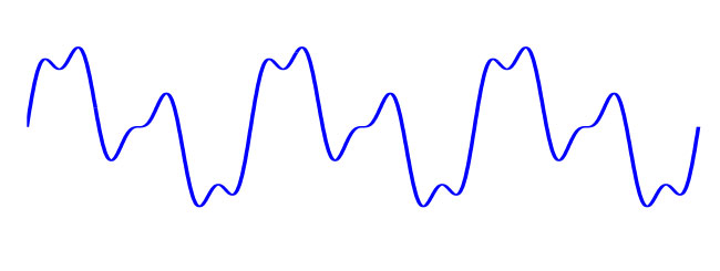
Figure 1: An arbitrary wave. Three cycles (periods) of the wave are shown. The shape of the repeating unit defines the timbre.
Note that the same shape is repeated three times in the waveform in Figure 1. The frequency at which the waveform repeats itself defines the pitch of the sound, while the shape of that waveform defines the timbre.
It turns out that the shape of the waveform comes from the existence of harmonic vibrations or overtones, which are vibrations at exactly twice, three times, four times, etc. the pitch frequency (which is also called the fundamental frequency). Noisy and atonal instruments, like cymbals, have messier harmonics and often a poorly defined pitch, as a result of having continuous frequencies between the harmonics coming into play.
Waves can be added together. This is what is happening when a single speaker ends up sounding like an entire orchestra. The microphones recorded the sum of all the sound waves, and the speaker plays the sum back. I made the waveform in Figure 1 by arbitrarily adding together a few (sinusoidal) harmonics, as shown in Figure 2.
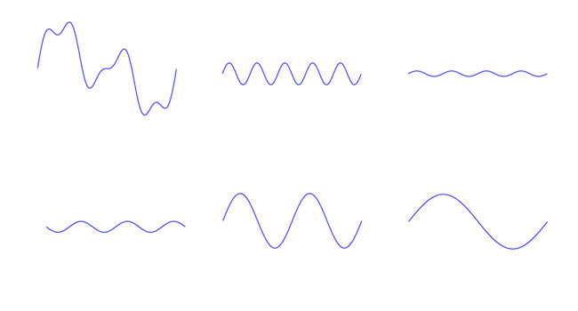
Figure 2: Building Timbre from Sinusoidal Waves
This building up of timbre in sounds by adding together waveforms is called synthesis. The same way we can synthesize waveforms with timbre by adding together harmonic waves, we can also analyze which harmonics make up a sound with timbre.
Noise and inharmonic sound.
Inharmonic sound departs from the ideas in the previous section, and the timbre contains frequencies away from the harmonic series (multiples of the fundamental or pitch frequency). Different sounds are inharmonic to different degrees. A bell or chime still conveys a certain pitch, however, when you sweep a filter across these instruments, you can hear that there are inharmonic frequencies participating in the sound.
Noise has a high degree of inharmonic content. White noise isn’t harmonic at all. It has equal amplitude at all frequencies and so there is no harmonic series there to talk about. One of the great things about white noise, is that you can pick out any pitch that you want using a narrow bandpass filter (we’ll get more into filters in the ‘Filters and Equalizers’ section). This is used to create nice sweeping sounds and sci-fi radio-transmission style glitches, when the frequency of the filter is swept across the noise. You can also get some good percussion samples using bandpass filtered noise as your input.
Amplification and Fidelity
When a signal passes through an amplifier, two things are added: noise and distortion. Keep in mind, the noise added by an amplifier won’t be simple white noise (as discussed in the previous section). For example, there will often be a hum at 50Hz to 60Hz; this comes from the AC power outlet. The hum coming from the power line usually has it’s own harmonics, and the spectrum of noise can be very far from being purely white.
Fidelity refers to the degree to which a signal is unaltered, or not distorted, as it passes through an amplifier. High fidelity (hi-fi) equipment does a good job of amplifying the signal without significant distortion. You can push both vacuum tube and solid-state (semiconductor) amplifiers into overdrive, resulting in a low fidelity (lo-fi) distorted (crunchy, fuzzy, static-sounding, harshly clipping, etc.) sound.
The change in texture that the lo-fi amplification imparts to your sound depends on the nature and quality of the amplification system. That wooly, warm distortion of a good tube amp is wonderful, and many other (sometimes inexpensive) lo-fi amps and effects can often be used to give an unusual character to sound in a recording or performance.
When distortion is introduced into a signal, additional harmonic content is gained. Overtones can be added to a sine wave by compressing or clipping it, and we will talk about the harmonic series of the square wave in the ‘’ section (which is like extreme clipping on a sine wave). Noise adds frequencies in between the harmonics.
When all of this works together, it can sound great; sometimes, attempts at lo-fi approaches can be less pleasant on the ear. Lo-fi or hi-fi. Mildly distorted or overdriven. Use your ear and give the song what it asks for.
Analog to Digital conversion.
Analog to digital conversion is a complex subject. However, we should touch on it here since it can definitely play an audible role in audio signal processing. Analog to digital conversion is the last step in the digital recording chain, before the digitized data is stored to computer memory. If this process is done right—with good quality converters, and the input preamps properly adjusted—the sound can be almost lossless.
This wasn’t always the case with early analog to digital converters, and a crummy analog to digital converter can really take away a lot of the hard work you put into finding that perfect timbre in the room.
When we digitize something, we are quantizing it (rounding it to discrete values) in both time and amplitude. Instead of a continuous analog waveform, now all we have is a bunch of digital data points of amplitude vs. time. So how can this actually get played back and sound the same as the analog (pre-digitized) signal? The short, somewhat hand-waving answer is that it is explained by Nyquist’s theorem, where if the highest frequency is sampled at least twice each period, everything works out OK.
I can give a qualitative description of Nyquist’s theorem here, hopefully enough to convey the ideas of good audio sampling, and the bad kind that leads to aliasing when high frequencies get ‘folded’ down and recorded as lower frequencies. When a signal is sampled at twice its frequency, it can be fully recovered during digital to analog conversion—if the amplitude resolution is good. This is shown in Figure 3.
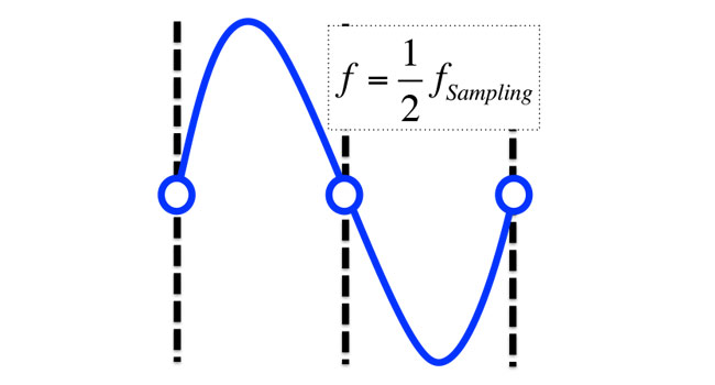
Figure 3: A sampled sine wave at the Nyquist frequency (half of the sampling frequency). This particular signal is also synchronized perfectly and in phase with the sampling clock.
In reality, there will always be some shift in the waveform (called phase) between the sampling events and where the waveform hits zero, and Figure 4 includes an arbitrary phase shift to illustrate this.
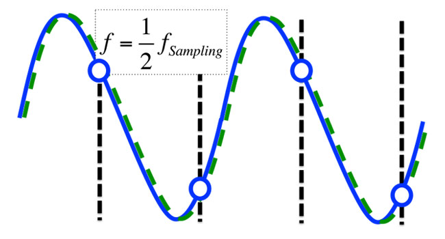
Figure 4: A sampled sine wave at the Nyquist frequency. This signal is not in phase with the sampling clock.
The dotted green line shows the lowest frequency sine wave that can accommodate the sampled points, meaning that the proper waveform will be reproduced on replay. Notice that for a waveform where we are below the Nyquist frequency, the situation is even better. Again, the lowest frequency solution is the right one (as shown in Figure 5).
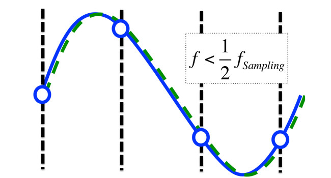
Figure 5: Signals with frequencies below the Nyquist frequency are sampled without loss.
When we try to sample a signal that exceeds the Nyquist frequency, as shown in Figure 6, you find that there is a lower frequency sine wave that satisfies the conditions of the digital data points. This means that that frequency will actually be reproduced at the lower frequency. This error in the frequency is called aliasing (or folding, since it folds down to lower frequencies).
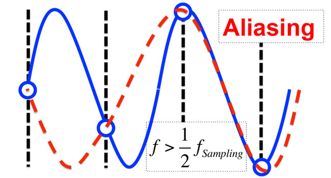
Figure 6: When the signal frequency exceeds the Nyquist frequency, the wave is ‘aliased’ down to a lower frequency, and the signal is not accurately recorded.
If we ensure that the sampling frequency is at least twice our maximum frequency entering the system, then all frequencies in the signal should be properly resolved in the frequency dimension,as long as the signal is strong enough.
There is still the aspect of digitization that we haven’t discussed, which is amplitude quantization. In the previous example, a perfect amplitude measurement was implied. In reality, an analog to digital converter rounds this amplitude to the closest binary value. In a 16-bit recorder, there are 216 (aka 65,536) binary values for amplitude. So this gives a pretty accurate representation if you fill the entire bank of binary values!
When you exceed the bit-depth (i.e. the 65,536 binary values) with a signal that is too strong, you get digital clipping. This can be awful sounding, especially in poorly designed analog to digital converters.
The trick lies in getting the preamp in the sweet spot so that you aren’t clipping, but you are also filling your converter to get the most out of your resolution. The softer the signal is, the poorer your actual amplitude resolution gets. Compressing preamps, like tube amps, can let you clip the preamp to avoid clipping the analog to digital converter allowing you to really saturate that converter without fear of digital clipping.
Additive Synthesis
We already discussed how waves can be added together. This is the basis for additive synthesis. A square wave can be generated by adding together every odd harmonic (1st, 3rd, 5th, …) with the amplitude reduced by the harmonic number (i.e. 1,13,15,...), or mathematically:
But forget the mathematics, which really just describe the waveforms. You can see in Figure 7 that even with only 5 harmonics, we can get pretty close to a square waveform.
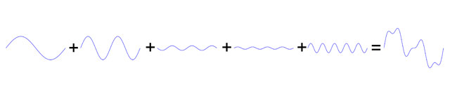
Figure 7: Adding together odd harmonics, each attenuated by their harmonic number (i.e. 1, 1/3, 1/5, etc ...), creates a square wave. The first five harmonics are shown here.
So to make an additive synthesizer, we need to be able to generate a whole bunch of harmonics and have some way of controlling their volume.
Additive synthesis is a very old technique, dating back to the use of pipe organs. Organ pipes do a pretty good job of giving relatively simple (almost sinusoidal) waveforms, and the drawbars determine how much air flows through each pipe giving the organist control over the timbre.
Additive synthesizers can produce really pleasing sounds, especially when the frequency and volume of the harmonics are modulated. Although the additive method gives great control over timbre, it is inherently bulky and expensive. However, with computational power continuing to rise, these limitations have been softened, and there are a lot of great software-based additive synthesizers on the market.
Filters and equalizers.
A filter changes the timbre of a sound by reducing or boosting the volume of each of its harmonics. Equalizers are made up of a variety of filters that can be used to manipulate timbre.
Two important filters are the high pass filter (HPF) and low pass filter (LPF). These filters attenuate everything above (for the LPF) and below (for the HPF) the cutoff frequency. These types of filters have control of resonance and roll-off. Roll-off controls are usually quantified by the degree of attenuation (in decibels) per octave (above/below the cutoff frequency). The resonance of the filter sets the amount of boost given to frequencies just below (for the LPF) and above (for the HPF) the cutoff frequency. Sweeping these types of filters across waveforms can give really nice timbres, and we will get into this more in later sections. High and low pass filters can be combined to give band pass filters that only let a defined band of sound through.
Equalizers allow you to amplify or attenuate the sounds at a variety of frequencies. Different equalizers have different capabilities, and can do a lot to modify timbres as well as making room for other instruments in a mix. You will find a parameter called Q, which is related to resonance and controls the breadth of the filter’s effect. Equalizers are handy tools for reducing the amount of noise present in signals recorded from lines or mics.
You can always bring a hard roll-off high pass filter right up to the lowest played note on a track, and you will eliminate nothing from the sound except noise and background racket. Extending the cutoff frequency of your high pass beyond the lowest fundamental begins to introduce a sort of low-fidelity sound (in the sense of an old radio), and plays games with the mind through creating a missing fundamental.
Adding a soft roll-off low pass filter can be used to tame back strong overtones, distortion, or even a certain degree and type of clipping. And, stronger filters can be used to strongly isolate tones. Harder roll-offs on low-pass filters can sound better when dealing with harsh synthesized tones like square waves, and can really create strong variations in the timbre as the cutoff frequency sweeps over the overtones.
By cranking up the resonance, or Q, on a filter, you can quickly hear it’s effect. You will find a sci-fi sounding bump in the sound. Try sweeping the cutoff frequency around, and you will hear this resonance picking out harmonics and noise in between.
Unless you are doing something experimental, you’ll probably want to pull the resonance or gain at a particular frequency back to a nice subtle spot that makes the instrument fit into the mix. You can use manual automation of the resonance and cut-off frequencies to follow the dynamics of the song and get more experimental in particular spots of a song.
Subtractive Synthesis
An alternative to building up a complex timbre, one harmonic at a time, is to start out with a harmonically complex waveform and then use filters to achieve various timbres. This method is called subtractive since the filters remove harmonics from the signal in order to control timbre.
Figure 8 shows what the output of an ideal (i.e. very hard roll-off) low pass filter as it removes the last five harmonics from a square wave. Notice how the number of humps is equal to the number of harmonics present in the signal. You can imagine how the wave would become more square as you add more harmonics and get more humps.
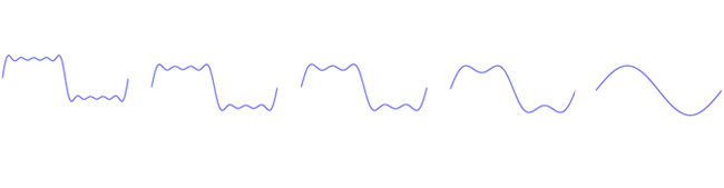
Figure 8: Low pass filtering a square wave changes its timbre, making the tone more pure. The top waveform shows a square wave that has been filtered down so that only 5 harmonics are left, and each subsequent waveform has one more overtone removed.
Subtractive synthesis requires at minimum a signal generator and a filter. As a result, subtractive synthesizers are much less demanding than additive synthesizers in terms of the hardware required to build one. Subtractive synths are ubiquitous in the electronic music world as a result.
Modulation
Acoustic sounds have timbres that changes over time. We can emulate this in synthesized sounds using modulation, which means we vary a particular attribute of the sound.
In an additive synth, we can have the powerful ability to modulate both the amplitude (volume) and frequency of each harmonic. Subtle modulation of the frequency of each overtone at different rates and amplitudes can have some really interesting effects.
With subtractive synthesis, we can only modulate the total volume and the attributes of any filters or effects that the input waveform is conditioned by. Even with these constraints, incredible sounds can be made with the use of envelopes, low frequency oscillators, and manual automation.
Envelopes
Envelopes output a control signal that changes over time and can be used to modulate the total amplitude, cutoff frequency, and any other attributes that the envelope is routed to control. Typical envelopes are of the Attack/Decay/Sustain/Release (ADSR) type, as illustrated in Figure 9. This is a powerful, albeit somewhat confusing, system that can take some getting used to because attack, decay and release define times, while sustain defines a level.
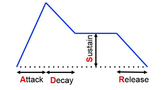
Figure 9: An ADSR (Attack, Sustain, Decay, Release) style envelope, which can be used to modulate all sorts of things.
Low Frequency Oscillator
Low frequency oscillators (LFOs) allow another waveform to modulate the attributes of a sound. The low frequency of an LFO means that the attribute being modulated changes very slowly relative to the audio frequency signal. This can create slowly or quickly evolving effects. LFOs can be routed to control parameters like amplitude (tremolo), frequency (vibrato), and filter cut-off (giving a sort of auto-wah effect). You may also find LFOs useful for creating stereo space as well by routing the LFO to the pan of a signal (auto-pan).
Vocoders
Vocoders are a type of modulator. In a typical vocoder, the “carrier signal” is split into a bunch of different bands (the number of bands changes the sound significantly). A "modulator signal" is then used to modulate the amplitude of each of the bands of the carrier wave. As a result, you can play a melody or chords on one instrument as the carrier, and whisper words into a microphone to modulate, and get that vocoder vocal effect.
You can get creative with what you use as your carrier and modulator signals. I have had a lot of fun routing my drum tracks, or silent drum tracks, to the modulator signal of a vocoder. This technique can be used to give a kind of atmosphere around your drum track, or can (by adding another silient drum track) be used to draw a more percussive timbre from a synthesizer waveform. You’ll have much better luck with vocoding if you start with waveforms that are harmonically complex (square-waves, sawtooths, etc.).
Automation
When dealing with software synthesizers, and digital audio workstations, changes in parameters (e.g filter cutoff) can be programmed into the song. This process is called automation. One way to do this, is to pencil in the variations that you want to have in your song. For example, you could increase a low pass filter cutoff linearly throughout a build in a track to let those higher harmonics progressively leak through and buid energy by just drawing in two points on your automation curve.
A great, and more organic alternative to hard programming in your automations is to live record them. This means using whatever you have (the mod wheel on your synth, external control knobs, a tablet, or a computer mouse) to control your parameters while you record the changes that you make while the song is running through. This takes a little extra time, but it gives a great degree of humanity to music and I always appreciate when I hear that care in music.
As a side note, the idea of manual automation is also really useful in creating stereo space, as well as the harmonic space that we have been focusing on here. You can extend this to manually automating the dry and wet control on your reverb to convey forward and backward motion, and the pan knob to create left to right motion. Try controlling the two of these at the same time – something that could also be done using an XY pad.
Samplers
Samplers can have a lot of the same filter features as a subtractive synthesizer; however, the input waveform is instead a sample. A sampler takes any recorded chunk of sound, and pitch shifts it across the keyboard so that it can be played like a synth. A little bit of care in the tuning, and some great sounds can come about.
You can get really creative here with sounds around the house, and adding a bit of portomento (amount of time spent sliding between notes) can really create some interesting effects. Some samplers allow for velocity crossfading, which can let you record two or more samples with different timbres so that the harder a key is hit, the more the other timbres ring through. These attributes of a sampler, mixed with amplitude and filter modulation really open up a world of possibilities for both live and recorded music.
Sterile and dynamic timbres.
We aren’t used to hearing static tones (that have perfectly constant timbre) in nature. Acoustic sounds have timbre that is always evolving in a complex way over time. Synthesizers can produce sterile sounding tones if the timbre is not modulated, almost like someone speaking in monotone. Sometimes a sterile sound can work out great in a song, especially with some sympathetic effects or acoustic sound treatments, and there is always this expressive freedom to make the decision. Think of it like a spectrum.
When you record an acoustic sound, the timbre is inherently dynamic. To get expressive sounds that evolve in timbre out of a synthesizer can take quite a bit of time and effort, until you get over that learning curve. Once you become comfortable with various means of modulation, you will find that you can get expressive timbres out of synthesizers without too much bother.
With a subtractive synth, it really helps to have an input waveform that already has some timbral evolution. Samplers are great for this, as they have the filters, envelopes, and LFOs of a subtractive synthesizer, but can have really nice dynamic samples as the input waveform. With a static input waveform, the filter cutoff and volume can be modulated (manually, or via envelopes and LFOs) to achieve dynamic timbres.
If you start playing around with manual automation of parameters on your synth, or even do live recordings & performance with synths where you tweak these knobs on the fly, you will find that synthesizers and samplers can be used to achieve expressive sounds that can give your live performance or studio recordings a whole new dimension.
Generating nice dynamic timbres, or preserving those recorded from acoustic instruments is crucial to creating expressive music that engages the listener. These sounds are welcoming and keep drawing us into the music, especially when the modulations keep moving and don’t get too loopy throughout the track. If you are wanting to use sterile tones and unchanging loops in your songs for artistic purposes, try weaving some modulations that evolve throughout the track and some instruments with dynamic timbres in with these to keep an overall sense of motion in your track. The spectrum between the two concepts always gives you room to find the balance that suits your vision.
Martin Gerber is working towards a PhD in Engineering Physics focused on solar energy research. He also skateboards, produces multi-genre music and plays in the band Stereography (vocals, guitar, and keys).